library(tidyverse) # for data management and plotting
library(ggpubr)
library(gtsummary) # for the nice tables
library(ggdist) # for the "half-violin" plot (stat_slab)
pen <- palmerpenguins::penguinsHW 07: Bivariate Modeling A
Two Sample T-Test and ANOVA
Purpose
We’ve been visually exploring relationships between two variables by creating appropriate plots to assess how the distribution of a primary outcome (response/dependent) variable changes according to the level of a predictor (explanatory/independent/covariate) variable. We can learn a lot by conducting exploratory data analysis, and if description is the goal then this is where your work can stop.
However, if you want to make conclusions or inference about a relationship, then formal statistical analysis techniques are needed. We start here by formally testing if relationships or associations between two measures exist, then later will see how additional third variables can potentially disrupt or enhance any association that you may find.
Submission instructions
- Use the QMD template answer the questions.
- Upload a PDF of your work to the assignment to Gradescope via Canvas
Instructions
In this assignment you will practice TWO(2) different types of bivariate analysis:
- (Q~B) Quantitative Outcome ~ Binary Categorical Explanatory == Two-sample t-tests for a difference in means
- (Q~C) Quantitative Outcome ~ Categorical Explanatory == ANOVA
For each analysis you will do the following steps. Follow the examples in the course notes and at the bottom of this assignment for guidance on how to complete each step.
Identify response and explanatory variables.
- State which variable (including the variable name from your codebook) will be your explanatory variable and which will be your response variable.
- Remember, you have some variables in your codebook that can act as both categorical and quantitative.
- Decide which of those variables makes sense to “explain” the other. Don’t just blindly pick a bunch of variables.
- Think about the relationship among your variables, keeping in mind your original research questions. You may use gender as your categorical explanatory variable if you are struggling to find an explanatory and response relationship that makes sense.
Visualize and summarize the bivariate relationship Create an appropriate bivariate plot to visualize the relationship you are exploring. Calculate appropriate summary statistics. Summarize the relationship between the explanatory and outcome variables in short paragraph form. This is similar to what you did in HW5.
Write the null and research hypothesis in words and symbols.
- Define the parameters being tested. (\(\rho\), \(p_{1}\), \(\mu_{1}\), \(\rho_{1}\) etc)
- Translate the null and alternative hypotheses into \(H_{0}\) and \(H_{A}\) with symbols.
Identify, justify, and perform the analysis
- Even if these assumptions are potentially violated, for the purposes of this assignment, acknowledge this limitation and continue with the prescribed analysis.
- If the ANOVA is significant - follow up with a Tukey HSD post hoc comparison and discuss which groups are different.
Assess the evidence and make a conclusion.
- State your final conclusion in a full English sentence in the context of the research hypothesis using no symbols or statistical jargon.
- Your conclusion must contain a point estimate, CI for that point estimate and a pvalues.
Example: (Q ~ B) Two sample T-Test for Independent Groups
We would like to know, is there convincing evidence that the average body mass differs between male and female penguins?
1. Identify response and explanatory variables
- Sex = binary explanatory variable (variable
sex) - Body mass = quantitative response variable (variable
body_mass_g)
2. Visualize and summarise bivariate relationship
plot.mass.sex <- pen %>%
  select(sex, body_mass_g) %>%
  na.omit()

plot.mass.sex %>%
  ggviolin(
    x = "sex",
    y = "body_mass_g",
    color = "sex",
    add = c("mean", "boxplot")
  ) +
  color_palette(palette = "jco") +
  xlab("Sex")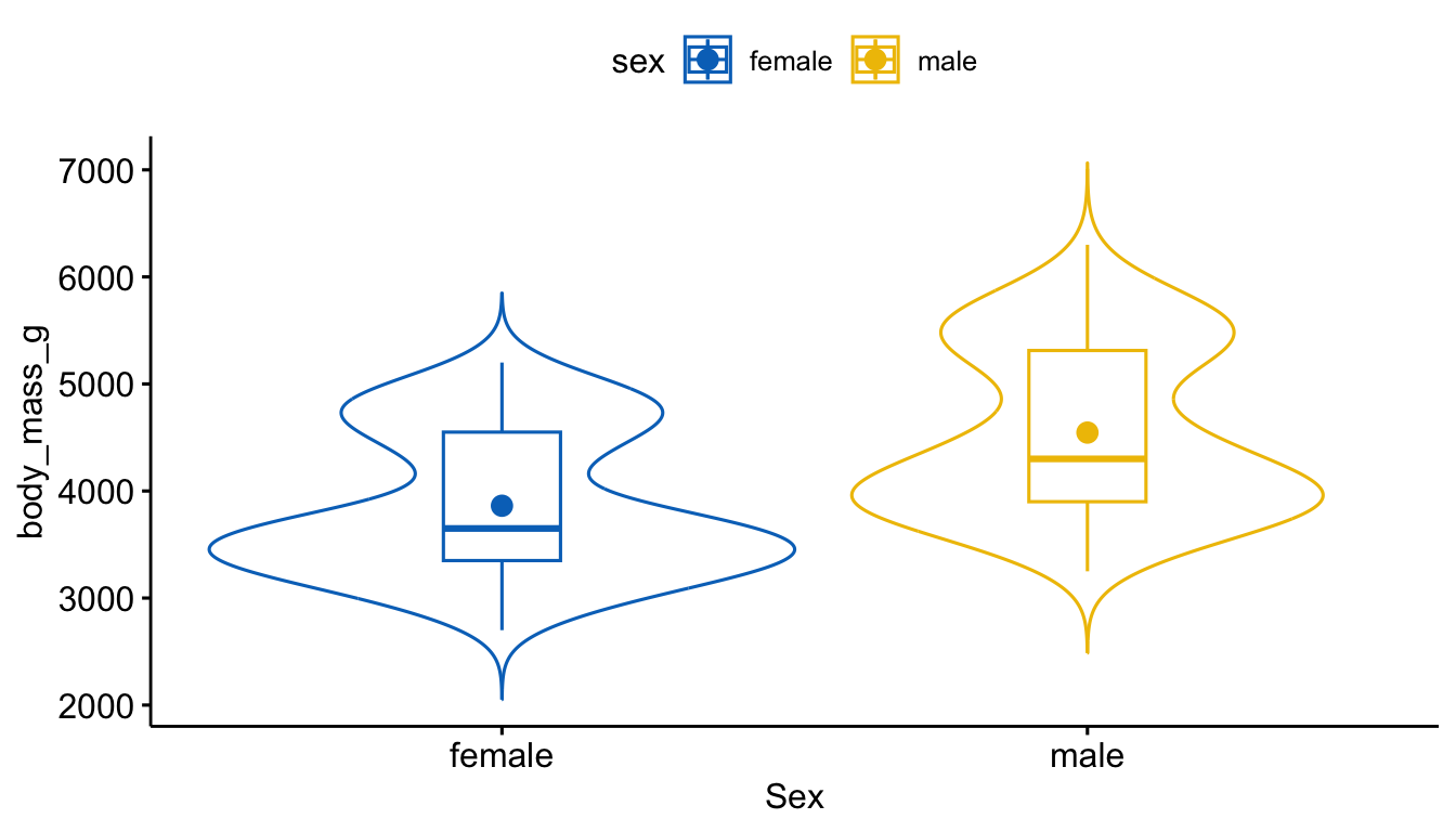
pen %>%
  tbl_summary(
    include = "body_mass_g",
    by = "sex",
    digits = all_continuous() ~ 1,
    statistic = list(
      all_continuous() ~ "{mean} ({sd})"
    )
)| Characteristic | female N = 1651 |
male N = 1681 |
|---|---|---|
| body_mass_g | 3,862.3 (666.2) | 4,545.7 (787.6) |
| 1 Mean (SD) | ||
Female penguins have an average body mass of 3,862.3 g (SD = 666.2), while male penguins average 4,545.7 g (SD = 787.6). Males are higher in center by about 680 g and show slightly more variability. Both distributions appear bimodal with no clear skew.
3. Write the null and research hypothesis in words and symbols.
Let \(\mu_f\) be the average body mass for female penguins, and \(\mu_m\) be the average body mass for male penguins.
\(H_{0}: \mu_{m} - \mu_{f} = 0\) There is no difference in the average body mass between female and male penguins.
\(H_{A}: \mu_{m} - \mu_{f} \neq 0\) There is a difference in the average body mass between female and male penguins.
4. Identify, justify, and perform the analysis
- We are comparing means between two independent groups → use a Two-Sample T-Test.
- Independence is reasonable since each penguin is only in one group.
- Distributions are bimodal but not skewed, so no major concerns, and sample sizes are large enough to rely on the CLT.
- Observations are independent (each penguin is a separate case).
- Standard deviations are similar (787.6 / 666.2 < 2).
t.test(body_mass_g ~ sex, data = pen)
    Welch Two Sample t-test

data:  body_mass_g by sex
t = -8.5545, df = 323.9, p-value = 4.794e-16
alternative hypothesis: true difference in means between group female and group male is not equal to 0
95 percent confidence interval:
 -840.5783 -526.2453
sample estimates:
mean in group female   mean in group male
            3862.273             4545.685
5. Assess the evidence and make a conclusion.
The p-value is very small so we would reject the null in favor of the alternative hypothesis.
There is sufficient evidence to conclude that male penguins weigh significantly more on average than females, by 683.4 (526.2, 840.6) grams (p < .0001).
Example: (Q ~ C) ANOVA
I would like to know if there is a difference in the average flipper length between the three species of penguins.
1. Identify response and explanatory variables
- Species = categorical explanatory variable
- Flipper length = quantitative response variable
2. Visualize and summarise bivariate relationship
ggplot(pen, aes(x=flipper_length_mm, y=species, fill=species)) +
stat_slab(alpha=.5, justification = 0) +
geom_boxplot(width = .2, outlier.shape = NA) +
geom_jitter(alpha = 0.5, height = 0.05) +
stat_summary(fun="mean", geom="point", col="red", size=4, pch=17) +
theme_bw() +
labs(x="Flipper Length (mm)", y = "Species") +
theme(legend.position = "none")
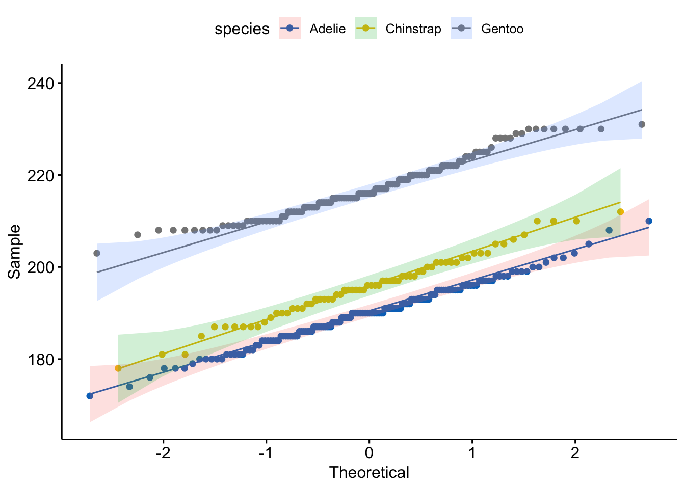
ggqqplot(pen,
x = "flipper_length_mm",
color = "species") +
color_palette(palette = "jco")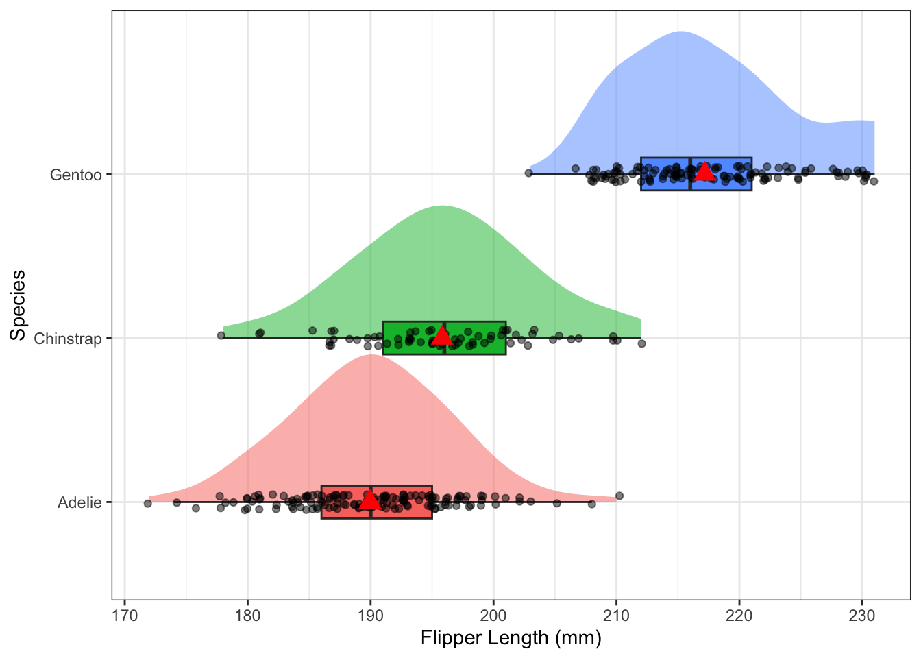
pen %>%
  tbl_summary(
    include = "flipper_length_mm",
    by="species",
    missing = "no",
    digits = all_continuous() ~ 1,
    statistic = list(
      all_continuous() ~ "{mean} ({sd})"
))| Characteristic | Adelie N = 1521 |
Chinstrap N = 681 |
Gentoo N = 1241 |
|---|---|---|---|
| flipper_length_mm | 190.0 (6.5) | 195.8 (7.1) | 217.2 (6.5) |
| 1 Mean (SD) | |||
The distribution of flipper length varies across the species, with Gentoo having the largest flippers on average at 217.2mm compared to Adelie (190mm) and Chinstrap (195.8mm). The distributions are normally distributed with very similar spreads, Chinstrap has the most variable flipper length with a SD of 7.1 compared to 6.5 for the other two species.
3. Write the null and research hypothesis in words and symbols.
- Null Hypothesis: There is no association between flipper length and species.
- Alternate Hypothesis: There is an association between flipper length and species.
Let \(\mu_{A}, \mu_{C}\) and \(\mu_{G}\) be the average flipper length for the Adelie, Chinstrap and Gentoo species of penguins respectively.
\(H_{0}: \mu_{A} = \mu_{C} = \mu_{G}\)
\(H_{A}:\) At least one \(\mu_{j}\) is different.
4. Identify, justify, and perform the analysis
We are comparing means from multiple groups, so an ANOVA is the appropriate procedure. We need to check for independence, approximate normality and approximately equal variances across groups.
- Independence: We are assuming that each penguin was sampled independently of each other, and that the species themselves are independent of each other.
- Normality: The distributions of flipper length within each group are fairly normal. The density plots resemble a bell curve, and the Q-Q plots show points that are mostly along the line.
- Equal variances: Both the standard deviation and IQR (as measures of variability) are very similar across all groups.
species.flipper.model <- aov(flipper_length_mm ~ species, data=pen)

species.flipper.model |> summary()
Df Sum Sq Mean Sq F value Pr(>F)
species 2 52473 26237 594.8 <2e-16 ***
Residuals 339 14953 44
---
Signif. codes: 0 '***' 0.001 '**' 0.01 '*' 0.05 '.' 0.1 ' ' 1
2 observations deleted due to missingnessspecies.flipper.model |> TukeyHSD() #because the overall model is significant Tukey multiple comparisons of means
95% family-wise confidence level
Fit: aov(formula = flipper_length_mm ~ species, data = pen)
$species
diff lwr upr p adj
Chinstrap-Adelie 5.869887 3.586583 8.153191 0
Gentoo-Adelie 27.233349 25.334376 29.132323 0
Gentoo-Chinstrap 21.363462 19.000841 23.726084 05. Assess the evidence and make a conclusion.
The pvalue is very small so we would reject the null in favor of the alternative. A follow up Tukey HSD shows that all species are significantly different than each other since the p-values for all pairwise comparisons are also small.
There is sufficient evidence to believe that the average flipper length is significantly different between the three species of penguins (p<.0001). Specifically Gentoo penguins have significantly longer flippers than Adelie 27.2 (22.8, 31.6)mm and (21.4, 95% CI 17.0-25.8) mm longer than Chinstrap (p<.0001). Additionally, Chinstrap penguins have on average 5.8mm (95% CI 3.6, 8.2)mm longer flippers compared to Adelie (p<.0001)