HW 08: Bivariate Modeling B

Chi-Square Test of Association and Correlation Analysis

Purpose

This is a continuation of the previous assignment, where you will practice two additional types of bivariate analysis. Specifically a Chi-Squared tests of association between two categorical variables, and a Correlation Analysis to assess the strength of a linear relationship between two quantitative variables.

Submission instructions

Use the QMD template answer the questions.
Upload a PDF of your work to the assignment to Gradescope via Canvas

Instructions

In this assignment you will practice TWO(2) different types of bivariate analysis:

(B~C) Binary Outcome ~ Categorical (or Binary) Explanatory == \(\chi^{2}\) test of Association.
(Q~Q) Quantitative Outcome ~ Quantitative Explanatory == Correlation analysis

For each analysis you will do the following steps. Follow the examples in the course notes and at the bottom of this assignment for guidance on how to complete each step.

Identify response and explanatory variables.
- State which variable (including the variable name from your codebook) will be your explanatory variable and which will be your response variable.
- Remember, you have some variables in your codebook that can act as both categorical and quantitative.
- Decide which of those variables makes sense to “explain” the other. Don’t just blindly pick a bunch of variables.
- Think about the relationship among your variables, keeping in mind your original research questions. You may use gender as your categorical explanatory variable if you are struggling to find an explanatory and response relationship that makes sense.
Visualize and summarize the bivariate relationship Create an appropriate bivariate plot to visualize the relationship you are exploring. Calculate appropriate summary statistics. Summarize the relationship between the explanatory and outcome variables in short paragraph form. This is similar to what you did in HW5.
Write the null and research hypothesis in words and symbols.
- Define the parameters being tested. (\(\rho\), \(p_{1}\), \(\mu_{1}\), \(\rho_{1}\) etc)
- Translate the null and alternative hypotheses into \(H_{0}\) and \(H_{A}\) with symbols.
Identify, justify, and perform the analysis
- Even if these assumptions are potentially violated, for the purposes of this assignment, acknowledge this limitation and continue with the prescribed analysis.
- For the Correlation Analysis also calculate and interpret the coefficient of determination (\(R^2\)) with 95% CI.
- For the \(\chi^2\) test of association, if the test is significant, calculate and interpret at least one residual.
Assess the evidence and make a conclusion.
- State your final conclusion in a full English sentence in the context of the research hypothesis using no symbols or statistical jargon.
- Your conclusion must contain a point estimate, CI for that point estimate and a pvalues.

library(tidyverse) # for data management and plotting
library(sjPlot) # for the nice plot
pen <- palmerpenguins::penguins

Example (C~C) \(\chi^2\) analysis

We would like to know, were all species measured equally across the three sampling years? That is, is there an association between year and species?

1. Identify response and explanatory variables

The categorical explanatory variable is island (variable years)
The categorical response variable is species (variable species)

2. Visualize and summarise bivariate relationship

plot_xtab(
  x = pen$year,
  grp = pen$species,
  margin = "row",
  show.total = FALSE
) + theme_bw()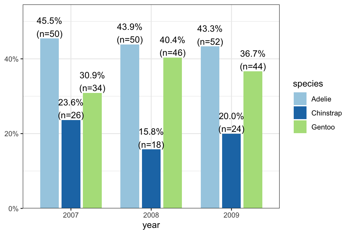

The distribution of penguin species is fairly similar across years. More Gentoo were observed in 2008 compared to other years (n=46, 40.4% vs 30.9% and 36.7% in 2007 and ’09 respectively), and fewer Chinstrap (n=18, 15.8% compared to 23.6 and 20% in 2007 and 2009 respectively).

3. Write the null and research hypothesis in words and symbols.

Let \(p_{A07}, p_{C07}, p_{G07}\) be the true proportions of Adelie, Chinstrap, and Gentoo penguins in 2007.

Let \(p_{A08}, p_{C08}, p_{G08}\) be the true proportions of Adelie, Chinstrap, and Gentoo penguins in 2008.

Let \(p_{A09}, p_{C09}, p_{G09}\) be the true proportions of Adelie, Chinstrap, and Gentoo penguins in 2009.

\(H_{0}:\) The species distribution (\(p_{Aj}, p_{Cj}, p_{Gj}\)) is the same in each year \(j\) (no association)

\(H_{A}:\) The species distribution differs for at least one year (association)

4. Identify, justify, and perform the analysis

A \(\chi^2\) test of association will be conducted. This is appropriate because both variables are categorical, and the expected cell counts are all greater than 5.

chisq.test(pen$year, pen$species)
chisq.test(pen$year, pen$species)$expected


    Pearson's Chi-squared test

data:  pen$year and pen$species
X-squared = 3.2156, df = 4, p-value = 0.5224

        pen$species
pen$year   Adelie Chinstrap   Gentoo
    2007 48.60465  21.74419 39.65116
    2008 50.37209  22.53488 41.09302
    2009 53.02326  23.72093 43.25581

5. Assess the evidence and make a conclusion.

The p-value is large so we would fail to reject the null.

There is not sufficient evidence to conclude that penguin species is associated with year. The species distribution appears to be similar across years (p=0.522).

Example (Q~Q) Correlation analysis

I am interseted in the relationship between the body mass and bill length of penguins.

1. Identify response and explanatory variables

The quantitative explanatory variable is body mass (g)
The quantitative response variable is bill length (mm)

2. Visualize and summarise bivariate relationship

ggplot(pen, aes(x=body_mass_g, y=bill_length_mm)) + 
  geom_point() + 
  geom_smooth(col = "red") +
  geom_smooth(method = "lm", col = "blue") + theme_bw()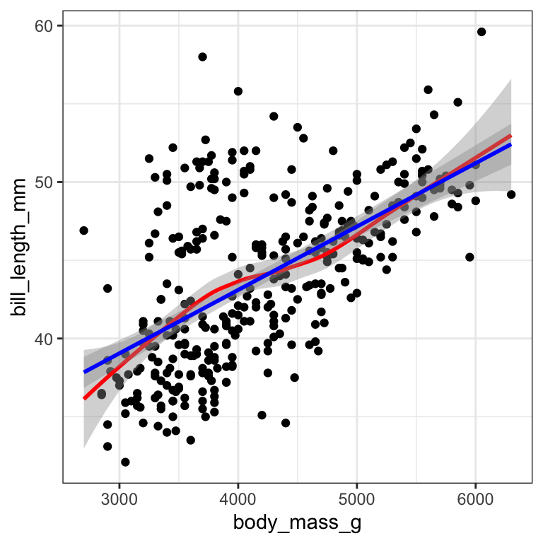

cor(pen$body_mass_g, pen$bill_length_mm, use = "pairwise.complete.obs")

[1] 0.5951098

There is a strong, positive, mostly linear relationship between the body mass (g) of penguins and their bill length (mm) (r=.595).

3. Write the null and research hypothesis in words and symbols.

Null Hypothesis: There is no correlation between the body mass and bill length of penguins.
Alternate Hypothesis: There is a correlation between the body mass and bill length of penguins.

Let \(\rho\) be the true correlation between body mass and bill length of penguins.

\(H_{0}: \rho=0\) There is no correlation.

\(H_{A}: \rho \neq 0\) There is a correlation

4. Identify, justify, and perform the analysis

Pearsons test of correlation will be conducted. This is appropriate because both variables are quantitative.
The relationship between variables are reasonably linear
The sample size is large.

cor.test(pen$body_mass_g, pen$bill_length_mm)


    Pearson's product-moment correlation

data:  pen$body_mass_g and pen$bill_length_mm
t = 13.654, df = 340, p-value < 2.2e-16
alternative hypothesis: true correlation is not equal to 0
95 percent confidence interval:
 0.5220040 0.6595358
sample estimates:
      cor 
0.5951098

5. Assess the evidence and make a conclusion.

The p-value is very small, there is sufficient evidence to reject the null and support the alternative.

# to calculate R^2 and the 95% CI
.595^2

[1] 0.354025

.522^2

[1] 0.272484

.659^2

[1] 0.434281

There was a statistically significant and strong correlation between the body mass (g) and bill length (mm) of penguins (r = 0.595, 95%CI .5220-.6595, p < .0001). The significant positive correlation shows that as the body mass of a penguin increases so does the bill length. These results suggest that 35% (95% CI: 27.2%-43.5%) of the variance in bill length can be explained by the body mass of the penguin.