HW 08: Multiple Linear Regression Modeling

Where most statistical modeling begins

Purpose

Fit a multiple regression model, assess model fit and interpret predictors of different data types.

Instructions

You will be fitting two linear regression models in this assignment. Both must have a quantitative predictor. The first will additionally have a binary predictor and the second model will have a categorical predictor containing more than 2 levels.

For each model you will do the following steps. Examples of each are provided below.

Identify variables in a sentence and variable names.
Write the mathematical model, defining each of your variables. For the binary and categorical variables you must include what each level of the variable means, indicating which one is the reference group. Double check this after you fit the model. If your reference group in the model is not the one stated here you will loose points.
Fit the multivariable model
Interpret all regression coefficients in a sentence that contains the point estimate \(b\), the confidence interval, and a p-value.
Graphically assess the model fit and comment on whether or not the assumptions of a regression model are upheld.

Submission instructions

Use the template provided: [QMD]
- Right click and ‘save as’, then upload this file into your scripts folder in Posit Cloud.
Upload your PDF to Canvas by the due date

library(tidyverse); library(gtsummary)
library(performance)
pen <- palmerpenguins::penguins

Part 1: Multiple Linear Regression with one quantitative and one binary predictor.

1. Identify variables

Quantitative outcome: Body Mass
Quantitative predictor: Flipper length
Binary predictor: Sex. This is an indicator of the penguin being male.

2. The mathematical model would look like:

\[ Y \sim \beta_{0} + \beta_{1}x_{1} + \beta_{2}x_{2}\]

Let \(y\) be body_mass_g
Let \(x_{1}\) be flipper_length_mm
Let \(x_{2}=0\) when sex='female'
Let \(x_{2}=1\) when sex='male'

3. Fit the multivariable model

pen.sex.model <- lm(body_mass_g ~ flipper_length_mm + sex, data=pen) 
tbl_regression(pen.sex.model, intercept = TRUE) %>% 
  add_glance_table(include = c("adj.r.squared", "nobs"))

Characteristic	Beta	95% CI¹	p-value
(Intercept)	-5,410	-5,973, -4,848	<0.001
flipper_length_mm	47	44, 50	<0.001
sex
female	—	—
male	348	268, 427	<0.001
Adjusted R²	0.805
No. Obs.	333
¹ CI = Confidence Interval

4. Interpret all regression coefficients of the multivariable model.

\(b_{0}\): For a female (sex=0) who has no flippers (flipper_length_mm=0), their predicted average body mass is -5410g (95% CI -5973, -4848)
\(b_{1}\): Holding penguin sex constant, for every additional mm longer a penguins flipper is, their predicted average body mass increases by 47mm (95% CI 44, 50). This is a significant association, p<.0001.
\(b_{2}\): Controlling for the length of a penguins flipper, the predicted average body mass for male penguins is 348g (268, 427) higher than for female penguins. This is a significant increase, p<.0001.

5. Assess model fit

check_normality(pen.sex.model) |> plot(type = "density") 
check_normality(pen.sex.model) |> plot(type = "qq") + 
  scale_y_continuous(limits = c(-3, 3))  
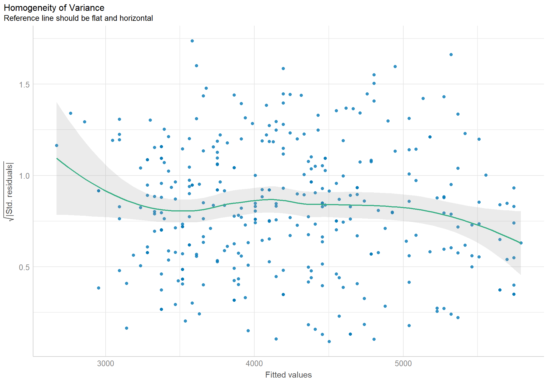
check_heteroscedasticity(pen.sex.model) |> plot()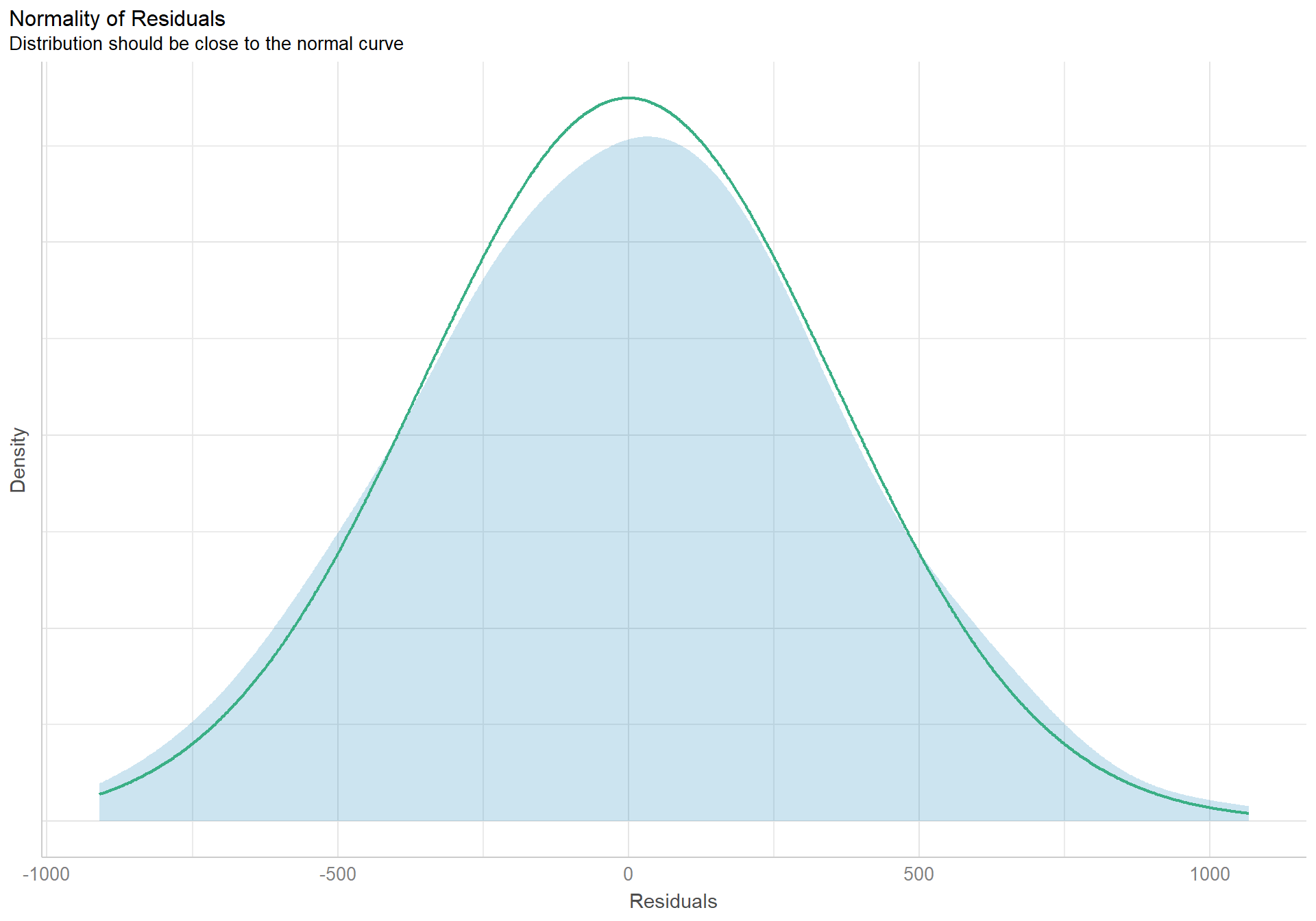

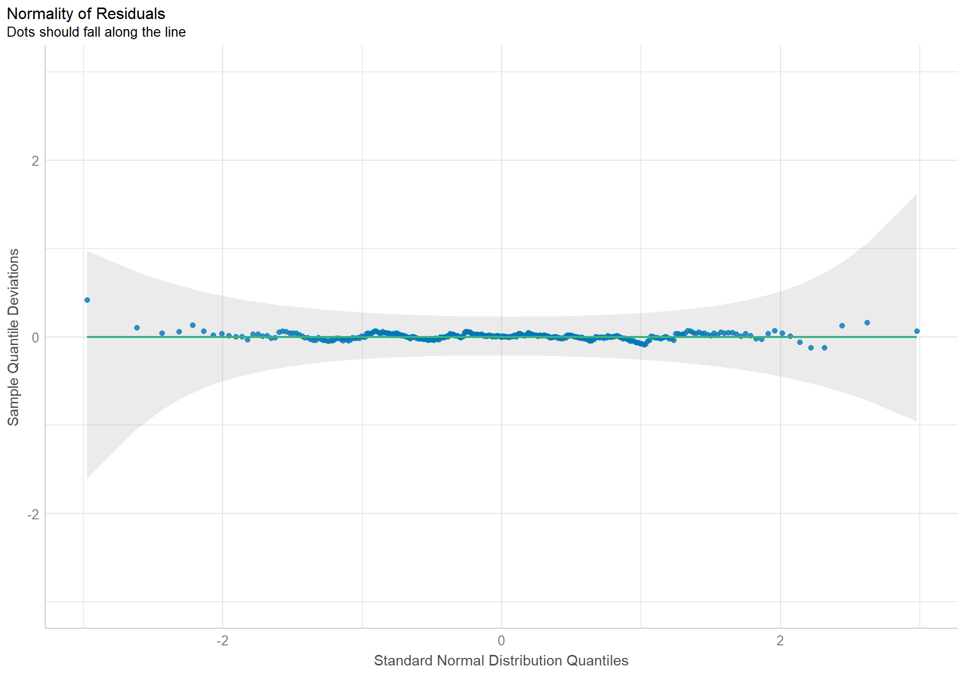
The density plot of the residuals looks like a nice pretty normal distribution, and the dots in the qqplot follow the reference line well.

The assumption of constant variance is also well enough upheld. The spike upward at the lower end of fitted values is being pulled up by a few outliers only, and the dip downward at the upper tail are all within normal amounts of variation.

Part 2: Categorical Predictor

1. Identify variables

Quantitative outcome: Body Mass
Quantitative predictor: Flipper length
Binary predictor: Island.

2. The mathematical model would look like:

\[ Y \sim \beta_{0} + \beta_{1}x_{1} + \beta_{2}x_{2} + \beta_{3}x_{3}\]

Let \(y\) be body_mass_g
Let \(x_{1}\) be flipper_length_mm
Let \(x_{2}=1\) when island='Dream' and 0 otherwise
Let \(x_{3}=1\) when island='Torgersen' and 0 otherwise

The reference group for Island is Biscoe.

3. Fit the multivariable model

pen.island.model <- lm(body_mass_g ~ flipper_length_mm + island, data=pen) 
tbl_regression(pen.island.model, intercept = TRUE) %>% 
  add_glance_table(include = c("adj.r.squared", "nobs"))

Characteristic	Beta	95% CI¹	p-value
(Intercept)	-4,625	-5,397, -3,853	<0.001
flipper_length_mm	45	41, 48	<0.001
island
Biscoe	—	—
Dream	-262	-370, -154	<0.001
Torgersen	-185	-323, -47	0.009
Adjusted R²	0.772
No. Obs.	342
¹ CI = Confidence Interval

4. Interpret all regression coefficients of the multivariable model.

\(b_{0}\): The predicted average body mass of a flipper-less penguin living on Biscoe island is -4625g (95% CI -5397, -3853)
\(b_{1}\): Controlling for the island, for every additional mm longer a penguins flipper is, their predicted average body mass increases by 45mm (95% CI 41, 48). This is a significant association, p<.0001.
\(b_{2}\): Controlling for the length of a penguins flipper, penguins on Dream island have on average 262g (154, 370) lower body mass than penguins living on Biscoe island. This is a significant difference, p<.0001.
\(b_{3}\): Controlling for the length of a penguins flipper, penguins on Torgersen island have on average 185g (47, 323) lower body mass than penguins living on Biscoe island. This is a significant difference, p=.0009.

5. Assess model fit

check_normality(pen.island.model) |> plot(type = "density") 
check_normality(pen.island.model) |> plot(type = "qq") + 
  scale_y_continuous(limits = c(-3, 3)) 
check_heteroscedasticity(pen.island.model) |> plot()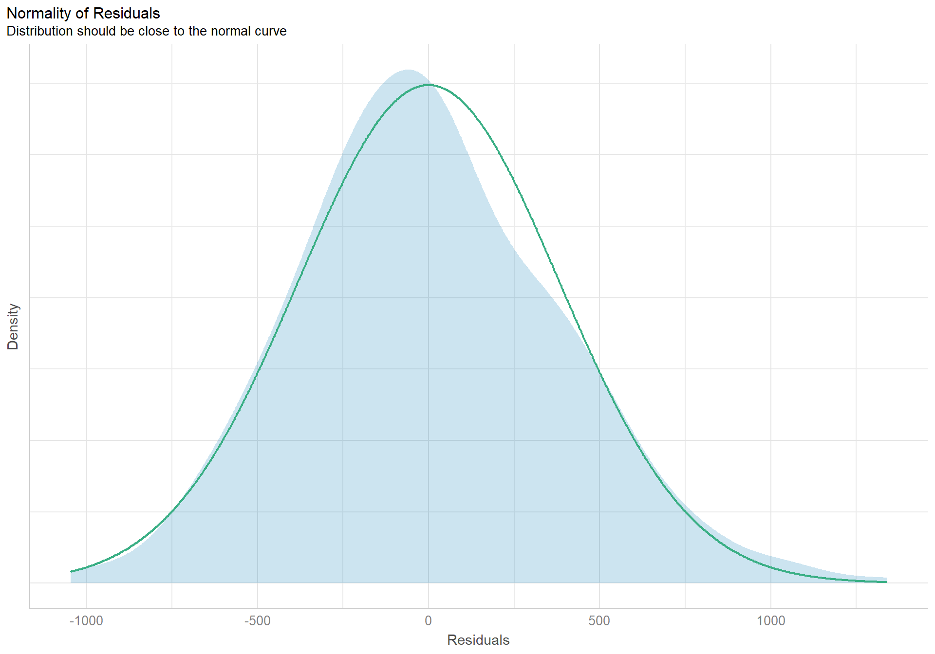

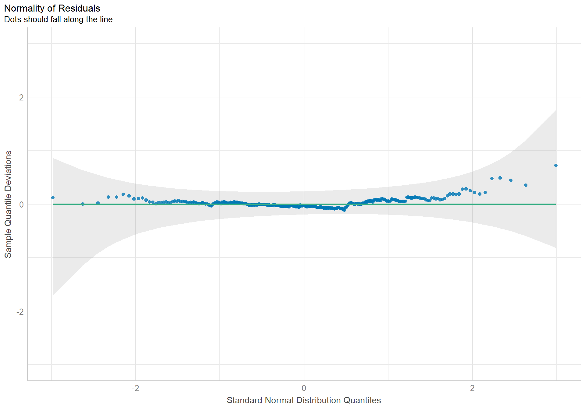
The density plot of the residuals looks like a nice pretty normal distribution, and the dots in the qqplot follow the reference line well.

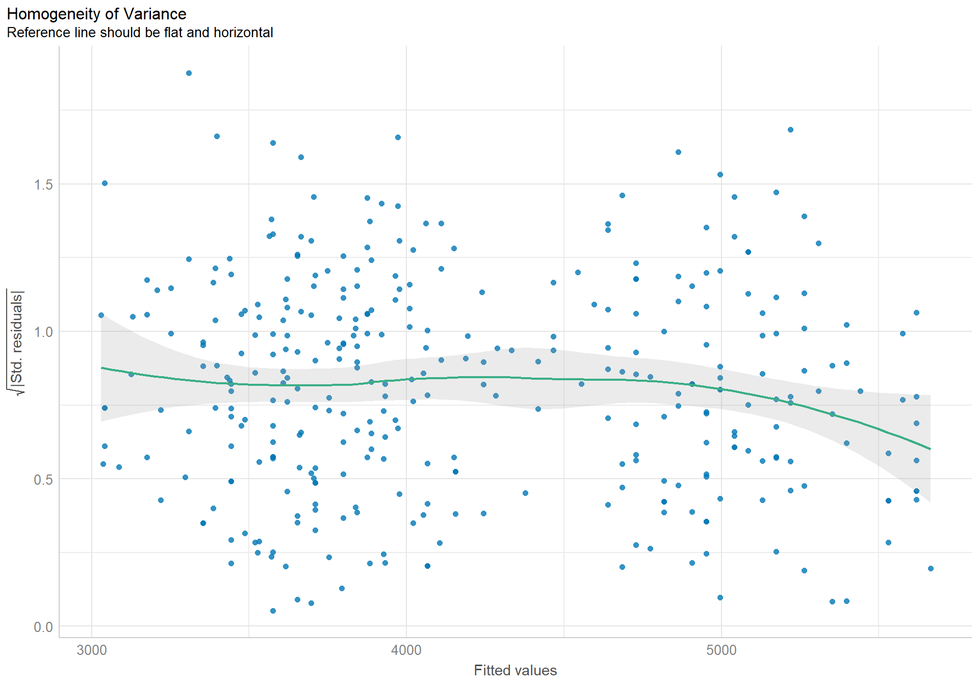
The assumption of constant variance is also well enough upheld. The slight curved patter is within normal amounts of variation.