# Load libraries
library(tidyverse)
library(ggdist)
library(sjPlot)
library(ggpubr)
library(gtsummary)
library(performance)

# Load raw data
raw <- read_csv(here::here("data/analytic_data2025_v3.csv"), skip = 1) %>%
janitor::clean_names()County-Level Conditions and Adult Health in the United States
Introduction
Background & Significance
We are interested in how county-level conditions are connected to adult health in the United States. Health is often talked about as something that mostly depends on individual choices, but counties can have very different conditions that may shape people’s health. We are especially interested in poor adult health and whether it is related to child poverty, high school completion, uninsured rates, and geographic region.
The sources we found show that county-level conditions like poverty, education, geography, and access to health care are all connected to how healthy people are. McCullough and Leider (2017) found that wealthier counties generally had better health outcomes, but wealth doesn’t explain everything. Dwyer-Lindgren et al. (2017) found large differences in life expectancy across U.S. counties, and socioeconomic and race/ethnicity factors explained about 60% of that variation. Bell and Owens-Young (2020) used County Health Rankings data with fair/poor self-rated health as the outcome and found that some associations differed by urban-rural classification, so geographic context matters. Yabroff et al. (2021) found that adults with no insurance or gaps in coverage had worse access to care and more trouble affording it, which is why we are looking at uninsured rates.
Research Questions
- Are county level child poverty rates associated with poor adult health?
- Are county level uninsured rates associated with child poverty rates?
- Are high school completion rates associated with poor adult health?
- Does county level uninsured rate differ by geographic region?
Methods
Study Design & Data Source
- The data come from the 2025 County Health Rankings & Roadmaps analytic dataset
- This is an observational study using secondary data.
- The unit of observation is a U.S. county.
- The population of interest is all U.S. counties.
Variables of Interest
All of the quantitative variables are percentages of the county.
poor_fair_health_pct(v002_rawvalue): percentage of adults reporting poor or fair health. Quantitative response variable for RQ1 and RQ3.child_poverty_pct(v024_rawvalue): percentage of children living in poverty. Quantitative explanatory variable for RQ1, quantitative response variable for RQ2.high_school_completion_pct(v168_rawvalue): percentage of adults with a high school diploma or equivalent. Quantitative explanatory variable for RQ3uninsured_pct(v085_rawvalue): percentage of people under age 65 without health insurance. Quantitative explanatory variable for RQ2, quantitative response variable for RQ4.region(created fromstate): U.S. Census region of the county. Categorical explanatory variable for RQ4.
Data Management
# Keep only county rows and the variables we need
mydata <- raw %>%
  filter(countycode != "000") %>%
  select(state,
    poor_fair_health = v002_rawvalue,
    child_poverty = v024_rawvalue,
    high_school_completion = v168_rawvalue,
    uninsured = v085_rawvalue)

# Convert proportions to percentages
mydata$poor_fair_health_pct <- mydata$poor_fair_health * 100
mydata$child_poverty_pct <- mydata$child_poverty * 100
mydata$high_school_completion_pct <- mydata$high_school_completion * 100
mydata$uninsured_pct <- mydata$uninsured * 100

# Region
mydata$region <- case_when(
  mydata$state %in% c("CT", "ME", "MA", "NH", "RI",
                      "VT", "NJ", "NY", "PA") ~ "Northeast",
  mydata$state %in% c("IL", "IN", "MI", "OH", "WI", "IA", "KS", "MN", "MO",
                      "NE", "ND", "SD") ~ "Midwest",
  mydata$state %in% c("DE", "DC", "FL", "GA", "MD", "NC", "SC", "VA", "WV",
                      "AL", "KY", "MS", "TN", "AR", "LA", "OK", "TX") ~ "South",
  mydata$state %in% c("AZ", "CO", "ID", "MT", "NV", "NM", "UT", "WY",
"AK", "CA", "HI", "OR", "WA") ~ "West")- The first row of the raw file is a set of labels, so we skipped it when reading the data in.
- The raw file also has national and state summary rows. We used
countycode != "000"to keep only the county rows, which leaves 3,152 counties. - Poor or fair health, child poverty, high school completion, and uninsured are stored as proportions, so we multiplied them by 100 to get percentages.
- We used
stateto create a 4-levelregionvariable (Midwest, Northeast, South, West) following the U.S. Census regions.
Statistical Analysis
The two research questions that we chose to further analyze are as follows:
- RQ2: Are county level uninsured rates (Q) associated with child poverty rates (Q)?
- Method: Linear Regression
- Parameter: Let \(\beta_{1}\) be the true slope that describes the change in the percentage of children in poverty as the uninsured rate increases.
- \(H_{0}: \beta_{1} = 0\) There is no linear relationship between the uninsured rate and child poverty.
- \(H_{A}: \beta_{1} \neq 0\) There is a linear relationship between the uninsured rate and child poverty.
- RQ4: Does county level uninsured rate (Q) differ by geographic region (C)?
- Method: Analysis of variance (ANOVA), possibly followed by Tukey HSD to see which regions differ.
- Parameters: Let \(\mu_{M}, \mu_{N}, \mu_{S}\) and \(\mu_{W}\) be the true mean uninsured rates for counties in the Midwest, Northeast, South, and West respectively.
- \(H_{0}: \mu_{M} = \mu_{N} = \mu_{S} = \mu_{W}\) There is no difference in the average uninsured rate across U.S. Census regions.
- \(H_{A}:\) At least one regional mean is different.
Results
Sample Characteristics
Poor or Fair Health (quant response RQ1 and RQ3)
gghistogram(mydata$poor_fair_health_pct, add_density = TRUE) +
  labs(title = "Histogram of Poor or Fair Health",
       x = "Poor or Fair Health (%)",
       y = "Number of Counties")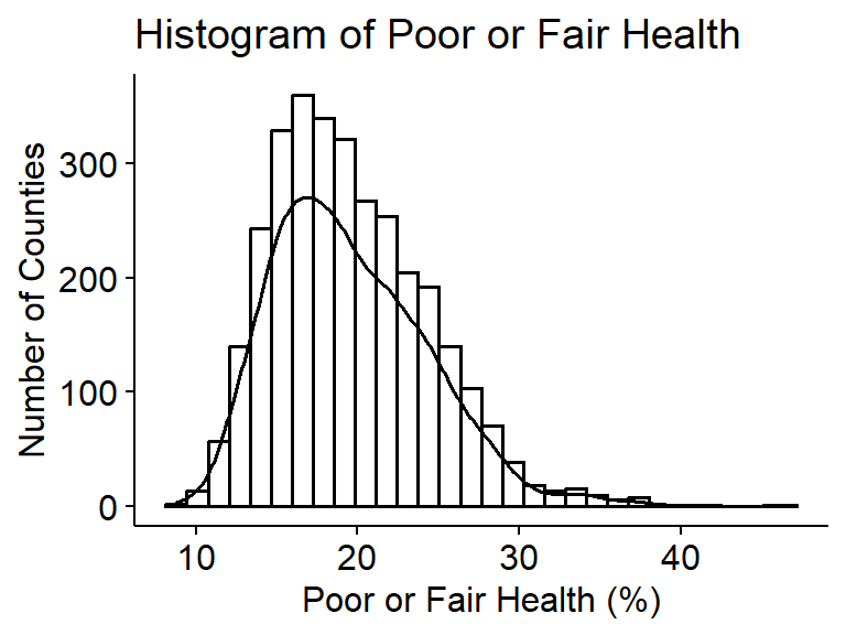
summary(mydata$poor_fair_health_pct) Min. 1st Qu. Median Mean 3rd Qu. Max. NAs
8.80 16.00 18.90 19.56 22.60 46.50 8 The percentage of adults in a county reporting poor or fair health is slightly right skewed with a median of 18.9% and mean of 19.6%. 50% of counties have between 16.0% and 22.6% of adults reporting poor or fair health, and the standard deviation is 4.8%.
Child poverty rates (quant explanatory RQ1, response RQ2)
gghistogram(mydata$child_poverty_pct, add_density = TRUE) +
  labs(title = "Histogram of Children in Poverty",
       x = "Children in Poverty (%)",
       y = "Number of Counties")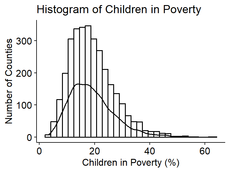
summary(mydata$child_poverty_pct) Min. 1st Qu. Median Mean 3rd Qu. Max. NAs
3.10 13.10 17.90 18.99 23.30 63.20 9 The percentage of children living in poverty is slightly right skewed with a median of 17.9% and mean of 19.0%. 50% of counties have a child poverty rate between 13.1% and 23.3%, and the standard deviation is 8.1%.
Uninsured rates (quant explanatory RQ2, response RQ4)
gghistogram(mydata$uninsured_pct, add_density = TRUE) +
  labs(title = "Histogram of Uninsured Rate",
       x = "Uninsured (%)",
       y = "Number of Counties")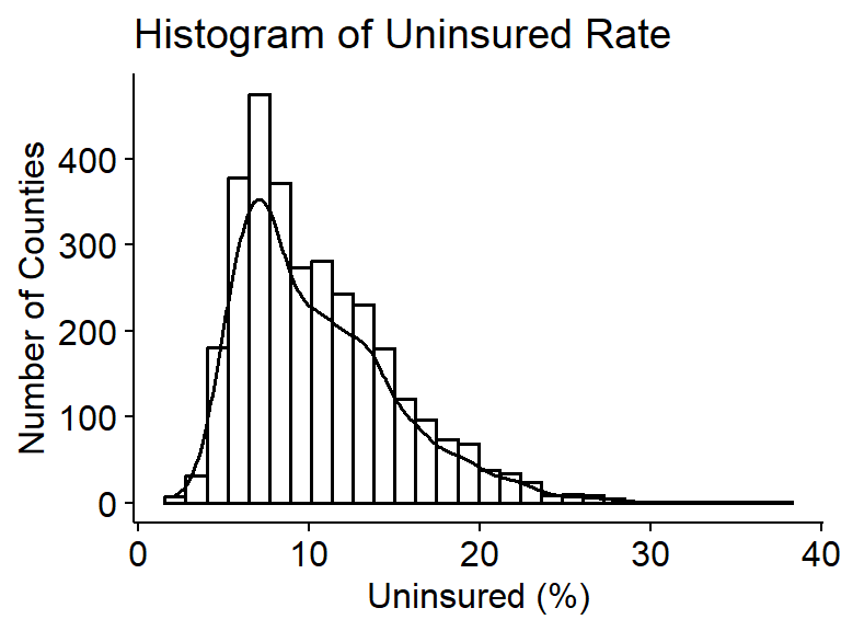
summary(mydata$uninsured_pct) Min. 1st Qu. Median Mean 3rd Qu. Max. NAs
2.149 6.919 9.411 10.473 13.176 37.681 9 The percentage of people under age 65 without health insurance is slightly right skewed with a median of 9.4% and a mean of 10.5%. 50% of counties have an uninsured rate between 6.9% and 13.2%, and the standard deviation is 4.7%.
High school completion rates (quant explanatory RQ3)
gghistogram(mydata$high_school_completion_pct, add_density = TRUE) +
  labs(title = "Histogram of High School Completion",
       x = "High School Completion (%)",
       y = "Number of Counties")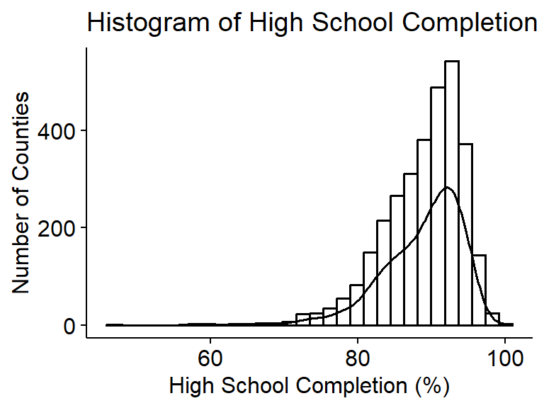
summary(mydata$high_school_completion_pct) Min. 1st Qu. Median Mean 3rd Qu. Max. NAs
46.81 85.65 89.91 88.76 92.75 100.00 8 The percentage of adults with a high school diploma or equivalent is slightly left skewed with a median of 89.9% and a mean of 88.8%. 50% of counties have a HS completion rate between 85.7% and 92.7%, and the standard deviation is 5.5%.
Geographic regions (Categorical explanatory RQ4)
plot_frq(mydata$region) +
  labs(title = "Distribution of Counties by Region",
       x = "Region",
       y = "Number of Counties") +
  ylim(c(0,1700))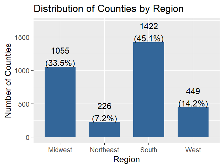
The South has the most counties, with 1,422 (45.1%), followed by the Midwest with 1,055 (33.5%) and the West with 449 (14.2%). The Northeast has the fewest, with 226 counties (7.2%).
Statistical Analysis
Are county level uninsured rates associated with child poverty rates? (RQ2)
ggplot(mydata, aes(x = uninsured_pct, y = child_poverty_pct)) +
  geom_point(alpha = .3) +
  geom_smooth(se = FALSE, col = "red") +
  geom_smooth(method = "lm", col = "black", se = FALSE) +
  theme_bw() +
  labs(title = "Child Poverty by Uninsured Rate",
       x = "Uninsured (%)",
       y = "Children in Poverty (%)")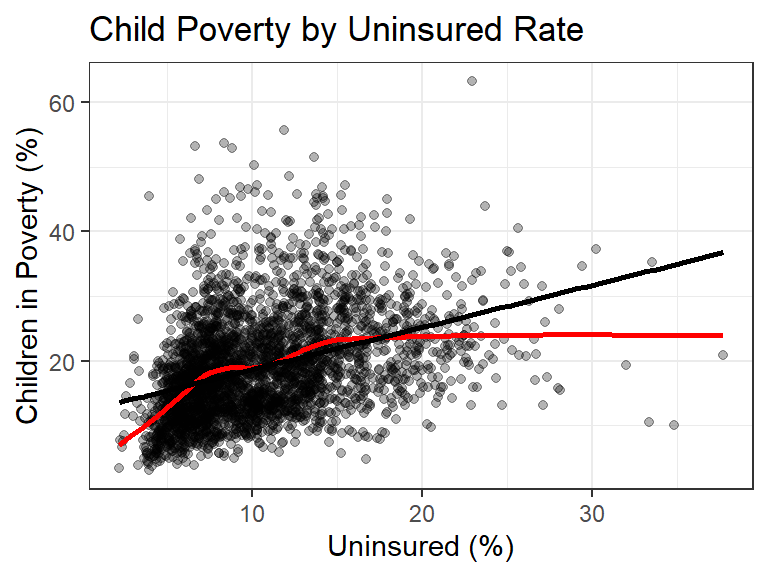
cor(mydata$uninsured_pct, mydata$child_poverty_pct, use = "pairwise.complete.obs")[1] 0.3762141There is a moderate, positive relationship between the uninsured rate and the percentage of children living in poverty (r = 0.38). Counties with more people uninsured tend to have more children in poverty. The red lowess line follows the regression line up to about 15% uninsured, but then levels off around 24% child poverty, so the straight line overestimates child poverty for the counties with the highest uninsured rates.
pov.unins <- lm(child_poverty_pct ~ uninsured_pct, data = mydata)
pov.unins |>
  tbl_regression(intercept = TRUE) |>
add_glance_table(include = r.squared)| Characteristic | Beta | 95% CI | p-value |
|---|---|---|---|
| (Intercept) | 12 | 12, 13 | <0.001 |
| uninsured_pct | 0.65 | 0.60, 0.71 | <0.001 |
| R² | 0.142 | ||
| Abbreviation: CI = Confidence Interval | |||
check_heteroskedasticity(pov.unins) |> plot()
check_normality(pov.unins) |> plot()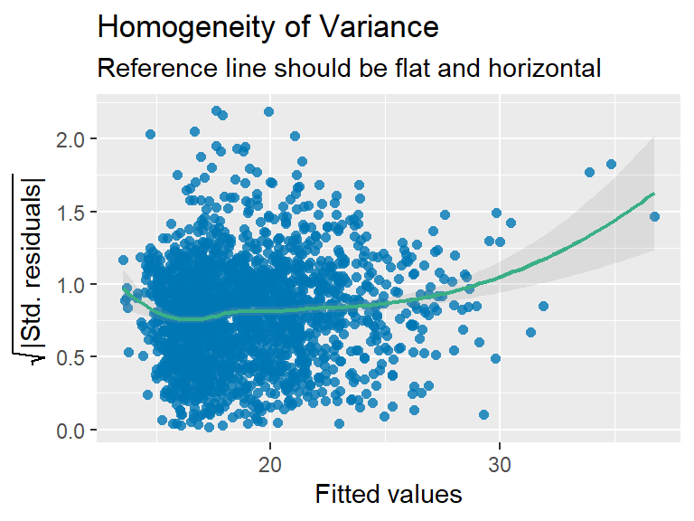
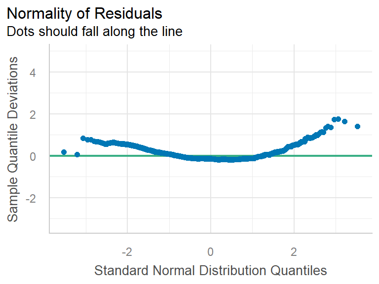
- Assumptions:
- Independence: Each row is a county, so we are treating counties as independent observations.
- Linearity: The relationship is roughly linear for most counties (below 15% uninsured), but it flattens out at the high end.
- Normality: The residuals curve away from the reference line at both ends, so they are right skewed and not normal.
- Constant variance: The reference line is fairly flat for most of the fitted values, but it curves up for the highest fitted values, so the variance is not constant.
- The sample size is large (3,143 counties), but since the assumptions are not fully met these results should be interpreted with some caution.
- Results:
- \(b_{0}\): A county with 0% of people uninsured would be expected to have about 12% of children living in poverty. No county actually has 0% uninsured (the lowest is 2.1%), so the intercept is not very meaningful on its own.
- \(b_{1}\): Each 1 percentage point increase in the uninsured rate is associated with a 0.65 (95% CI 0.60, 0.71) percentage point increase in child poverty on average (p < .001).
- \(R^2\): 14.2% of the variation in child poverty across counties can be explained by the uninsured rate.
- Conclusion: There is sufficient evidence of a positive linear relationship between the uninsured rate and child poverty in U.S. counties. For every 1 percentage point increase in the percentage of people under 65 without health insurance, the percentage of children living in poverty is 0.65 (95% CI 0.60, 0.71) percentage points higher on average (p < .001). However, the uninsured rate only explains about 14% of the variation in child poverty, and the relationship levels off for counties with the highest uninsured rates.
Does county level uninsured rate differ by geographic region? (RQ4)
ggplot(mydata, aes(x = uninsured_pct, y = region, fill = region)) +
  stat_slab(alpha = .5, justification = 0) +
  geom_boxplot(width = .2, outlier.shape = NA) +
  geom_jitter(alpha = .5, height = .05) +
  stat_summary(fun = "mean", geom = "point", col = "red", size = 4, pch = 17) +
  theme_bw() +
  labs(title = "Uninsured Rate by Region",
       x = "Uninsured (%)",
       y = "Region") +
  theme(legend.position = "none")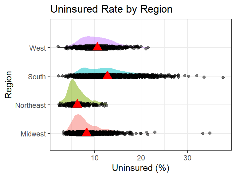
mydata |>
  select(region, uninsured_pct) |>
  na.omit() |>
tbl_summary(by="region")| Characteristic | Midwest N = 1,0551 |
Northeast N = 2181 |
South N = 1,4221 |
West N = 4481 |
|---|---|---|---|---|
| uninsured_pct | 7.4 (6.0, 9.8) | 5.8 (4.9, 7.3) | 12.2 (8.7, 15.7) | 10.3 (7.9, 12.8) |
| 1 Median (Q1, Q3) | ||||
The uninsured rate differs across U.S. regions. The South has the highest average uninsured rate at 12.7% (SD = 4.9), while the Northeast has the lowest at 6.2% (SD = 2.1). The West (10.6%, SD = 3.4) and Midwest (8.3%, SD = 3.2) fall in between. The South also has the most spread. All four regions are right skewed, and the Midwest has two high-end outliers above 33%.
ggqqplot(mydata, x = "uninsured_pct", color = "region")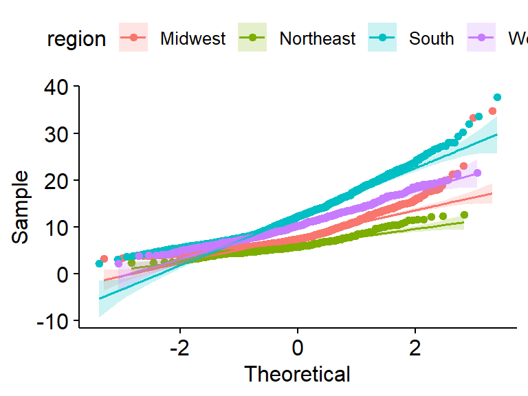
- Assumptions:
- Independence: Each row is a county, so we are treating counties as independent observations.
- Normality: The dots curve above the reference lines at the high end for every region, so the uninsured rate is right skewed within each region. However, the sample sizes are large (the smallest is the Northeast with 218 counties).
- Equal variances: The SD in the South (4.9) is more than double the SD in the Northeast (2.1), so the assumption of equal variances is likely not upheld. We proceed with the ANOVA but interpret the results with caution.
unins.region <- aov(uninsured_pct ~ region, data = mydata)
unins.region |> summary()
Df Sum Sq Mean Sq F value Pr(>F)
region 3 16280 5427 329.8 <2e-16 ***
Residuals 3139 51658 16
---
Signif. codes: 0 '***' 0.001 '**' 0.01 '*' 0.05 '.' 0.1 ' ' 1
9 observations deleted due to missingnessunins.region |> r2()# R2 for Anova Regression
R2: 0.240
adj. R2: 0.239unins.region |> TukeyHSD() Tukey multiple comparisons of means
95% family-wise confidence level
Fit: aov(formula = uninsured_pct ~ region, data = mydata)
$region
diff lwr upr p adj
Northeast-Midwest -2.031683 -2.807457 -1.255908 0
South-Midwest 4.460427 4.036723 4.884131 0
West-Midwest 2.300867 1.712850 2.888884 0
South-Northeast 6.492109 5.733672 7.250546 0
West-Northeast 4.332549 3.471465 5.193633 0
West-South -2.159560 -2.724507 -1.594613 0- Results: The ANOVA has F = 329.8 on 3 and 3139 degrees of freedom (p < .001), so we reject the null hypothesis. Region explains 24% of the variation in the uninsured rate (\(R^2\) = 0.24). The Tukey comparisons show that all six pairs of regions are significantly different from each other (p < .001). Counties in the South have an average uninsured rate that is 4.5 (95% CI 4.0, 4.9) percentage points higher than the Midwest, 6.5 (95% CI 5.7, 7.3) points higher than the Northeast, and 2.2 (95% CI 1.6, 2.7) points higher than the West.
- Conclusion: There is sufficient evidence that the average uninsured rate differs across U.S. Census regions (p < .001). Every region is different from every other region, with the South having the highest average uninsured rate and the Northeast having the lowest. Counties in the South have an average uninsured rate that is 6.5 (95% CI 5.7, 7.3) percentage points higher than counties in the Northeast.
Discussion & Conclusion
We found that counties with higher uninsured rates tend to have higher child poverty, and that the uninsured rate is different in every U.S. region. The relationship between uninsured rates and child poverty was positive but not very strong, since the uninsured rate explained only about 14% of the variation in child poverty. Region explained more of the variation in uninsured rates (24%), with Southern counties having the highest uninsured rates and Northeastern counties the lowest. These results fit with what we found in the literature. Yabroff et al. (2021) found that people without insurance have worse access to care, and our results show that uninsurance is concentrated in the South and in counties with more children in poverty, so these are the places most likely to face those barriers. McCullough and Leider (2017) found that wealthier counties had better health outcomes, and we found that poverty and uninsurance tend to show up in the same counties. Bell and Owens-Young (2020) found that geographic context matters, which matches the large differences we saw between regions.
Limitations
There are some limitations to this study. This is an observational study using county-level data, so we cannot say that being uninsured causes child poverty (or the other way around), and the results do not tell us about individual people. The assumptions for both analyses were not fully met. The regression residuals were right skewed with non-constant variance, the relationship leveled off at high uninsured rates, and the regions had unequal variances. We also did not account for other factors that could explain these patterns. For example, region could be related to both uninsured rates and child poverty, so it could be part of the reason the two are related. The uninsured measure only includes people under 65, and 9 counties were missing data. Overall, counties with more uninsured people tend to have more children in poverty, and where a county is located in the U.S. is strongly connected to how many of its residents are uninsured.
References
- University of Wisconsin Population Health Institute. (2025). County Health Rankings & Roadmaps 2025 analytic data [Data set]. County Health Rankings & Roadmaps. https://www.countyhealthrankings.org/health-data/methodology-and-sources/data-documentation
- Bell, C. N., & Owens-Young, J. L. (2020). Self-rated health and structural racism indicated by county-level racial inequalities in socioeconomic status: The role of urban-rural classification. Journal of Urban Health, 97, 52-61. https://doi.org/10.1007/s11524-019-00389-7
- Dwyer-Lindgren, L., Bertozzi-Villa, A., Stubbs, R. W., Morozoff, C., Mackenbach, J. P., van Lenthe, F. J., Mokdad, A. H., & Murray, C. J. L. (2017). Inequalities in life expectancy among US counties, 1980 to 2014: Temporal trends and key drivers. JAMA Internal Medicine, 177(7), 1003-1011. https://doi.org/10.1001/jamainternmed.2017.0918
- McCullough, J. M., & Leider, J. P. (2017). Associations between county wealth, health and social services spending, and health outcomes. American Journal of Preventive Medicine, 53(5), 592-598. https://doi.org/10.1016/j.amepre.2017.05.005
- Yabroff, K. R., Zhao, J., Halpern, M. T., Fedewa, S. A., Han, X., Nogueira, L., Zheng, Z., & Jemal, A. (2021). Health insurance disruptions and care access and affordability in the U.S. American Journal of Preventive Medicine, 61(1), 3-12. https://doi.org/10.1016/j.amepre.2021.02.014