# Load libraries
library(tidyverse)
library(ggdist)
library(sjPlot)
library(ggpubr)
library(gtsummary)

# Load raw data
raw <- read_csv(here::here("data/analytic_data2025_v3.csv"), skip = 1) %>%
janitor::clean_names()County-Level Conditions and Adult Health in the United States
Introduction
Background & Significance
We are interested in how county-level conditions are connected to adult health in the United States. Health is often talked about as something that mostly depends on individual choices, but counties can have very different conditions that may shape people’s health. We are especially interested in poor adult health and whether it is related to child poverty, high school completion, uninsured rates, and geographic region.
The sources we found show that county-level conditions like poverty, education, geography, and access to health care are all connected to how healthy people are. McCullough and Leider (2017) found that wealthier counties generally had better health outcomes, but wealth doesn’t explain everything. Dwyer-Lindgren et al. (2017) found large differences in life expectancy across U.S. counties, and socioeconomic and race/ethnicity factors explained about 60% of that variation. Bell and Owens-Young (2020) used County Health Rankings data with fair/poor self-rated health as the outcome and found that some associations differed by urban-rural classification, so geographic context matters. Yabroff et al. (2021) found that adults with no insurance or gaps in coverage had worse access to care and more trouble affording it, which is why we are looking at uninsured rates.
Research Questions
- Are county level child poverty rates associated with poor adult health?
- Are county level uninsured rates associated with child poverty rates?
- Are high school completion rates associated with poor adult health?
- Does county level uninsured rate differ by geographic region?
Methods
Study Design & Data Source
- The data come from the 2025 County Health Rankings & Roadmaps analytic dataset
- This is an observational study using secondary data.
- The unit of observation is a U.S. county.
- The population of interest is all U.S. counties.
Variables of Interest
All of the quantitative variables are percentages of the county.
poor_fair_health_pct(v002_rawvalue): percentage of adults reporting poor or fair health. Quantitative response variable.child_poverty_pct(v024_rawvalue): percentage of children living in poverty. Quantitative explanatory variable for RQ1, quantitative response variable for RQ2.high_school_completion_pct(v168_rawvalue): percentage of adults with a high school diploma or equivalent. Quantitative explanatory variable for RQ3uninsured_pct(v085_rawvalue): percentage of people under age 65 without health insurance. Quantitative explanatory variable RQ2 and 4.region(created fromstate): U.S. Census region of the county. Categorical explanatory variable for RQ4.
Data Management
# Keep only county rows and the variables we need
mydata <- raw %>%
  filter(countycode != "000") %>%
  select(state,
    poor_fair_health = v002_rawvalue,
    child_poverty = v024_rawvalue,
    high_school_completion = v168_rawvalue,
    uninsured = v085_rawvalue)

# Convert proportions to percentages
mydata$poor_fair_health_pct <- mydata$poor_fair_health * 100
mydata$child_poverty_pct <- mydata$child_poverty * 100
mydata$high_school_completion_pct <- mydata$high_school_completion * 100
mydata$uninsured_pct <- mydata$uninsured * 100

# Region
mydata$region <- case_when(
  mydata$state %in% c("CT", "ME", "MA", "NH", "RI",
                      "VT", "NJ", "NY", "PA") ~ "Northeast",
  mydata$state %in% c("IL", "IN", "MI", "OH", "WI", "IA", "KS", "MN", "MO",
                      "NE", "ND", "SD") ~ "Midwest",
  mydata$state %in% c("DE", "DC", "FL", "GA", "MD", "NC", "SC", "VA", "WV",
                      "AL", "KY", "MS", "TN", "AR", "LA", "OK", "TX") ~ "South",
  mydata$state %in% c("AZ", "CO", "ID", "MT", "NV", "NM", "UT", "WY",
"AK", "CA", "HI", "OR", "WA") ~ "West")- The first row of the raw file is a set of labels, so we skipped it when reading the data in.
- The raw file also has national and state summary rows. We used
countycode != "000"to keep only the county rows, which leaves 3,152 counties. - Poor or fair health, child poverty, high school completion, and uninsured are stored as proportions, so we multiplied them by 100 to get percentages.
- We used
stateto create a 4-levelregionvariable (Midwest, Northeast, South, West) following the U.S. Census regions.
Statistical Analysis
- RQ1:
- RQ2:
- RQ3:
- RQ4:
Results
Sample Characteristics
Poor or Fair Health (quant response)
gghistogram(mydata$poor_fair_health_pct, add_density = TRUE) +
  labs(title = "Histogram of Poor or Fair Health",
       x = "Poor or Fair Health (%)",
       y = "Number of Counties")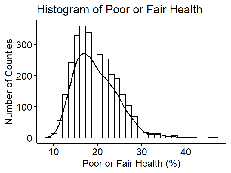
summary(mydata$poor_fair_health_pct) Min. 1st Qu. Median Mean 3rd Qu. Max. NAs
8.80 16.00 18.90 19.56 22.60 46.50 8 The percentage of adults reporting poor or fair health is centered around 18.9%, based on the median. The mean is 19.6%, which is slightly higher than the median, so the distribution appears slightly right-skewed, with 3 counties above 40%. The middle 50% of counties fall between 16.0% and 22.6%, and the standard deviation is 4.8%.
Child poverty rates (quant explanatory RQ1, response RQ2)
gghistogram(mydata$child_poverty_pct, add_density = TRUE) +
  labs(title = "Histogram of Children in Poverty",
       x = "Children in Poverty (%)",
       y = "Number of Counties")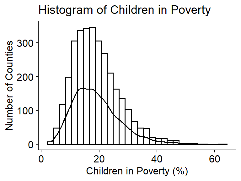
summary(mydata$child_poverty_pct) Min. 1st Qu. Median Mean 3rd Qu. Max. NAs
3.10 13.10 17.90 18.99 23.30 63.20 9 The percentage of children living in poverty is centered around 17.9%, based on the median. The mean is 19.0%, which is a little higher than the median, so the distribution appears slightly right-skewed, with 7 counties above 50%. The middle 50% of counties fall between 13.1% and 23.3%, and the standard deviation is 8.1%.
Uninsured rates (quant explanatory RQ2 and 4)
gghistogram(mydata$uninsured_pct, add_density = TRUE) +
  labs(title = "Histogram of Uninsured Rate",
       x = "Uninsured (%)",
       y = "Number of Counties")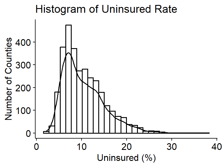
summary(mydata$uninsured_pct) Min. 1st Qu. Median Mean 3rd Qu. Max. NAs
2.149 6.919 9.411 10.473 13.176 37.681 9 The percentage of people under age 65 without health insurance is centered around 9.4%, based on the median. The mean is 10.5%, which is higher than the median, so the distribution appears right-skewed, with 6 counties above 30%. The middle 50% of counties fall between 6.9% and 13.2%, and the standard deviation is 4.7%.
High school completion rates (quant explanatory RQ3)
gghistogram(mydata$high_school_completion_pct, add_density = TRUE) +
  labs(title = "Histogram of High School Completion",
       x = "High School Completion (%)",
       y = "Number of Counties")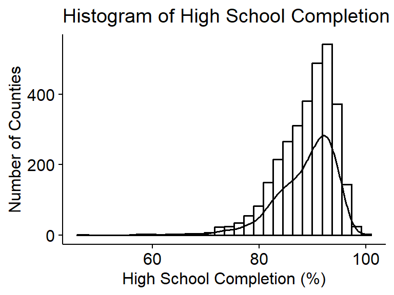
summary(mydata$high_school_completion_pct) Min. 1st Qu. Median Mean 3rd Qu. Max. NAs
46.81 85.65 89.91 88.76 92.75 100.00 8 The percentage of adults with a high school diploma or equivalent is centered around 89.9%, based on the median. The mean is 88.8%, which is lower than the median, so the distribution appears left-skewed, with 4 counties below 60%. The middle 50% of counties fall between 85.7% and 92.7%, and the standard deviation is 5.5%.
Geographic regions (Categorical explanatory RQ4)
plot_frq(mydata$region) +
  labs(title = "Distribution of Counties by Region",
       x = "Region",
       y = "Number of Counties")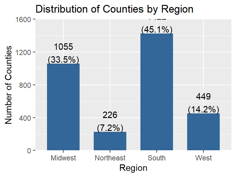
The South has the most counties, with 1,422 (45.1%), followed by the Midwest with 1,055 (33.5%) and the West with 449 (14.2%). The Northeast has the fewest, with 226 counties (7.2%). There are no missing values for region.
Statistical Analysis
RQ1
# Code for plot and summary statistics here- Description:
- Method:
- Assumptions:
- Results:
- Conclusion:
RQ2
# Code for plot and summary statistics here- Description:
- Method:
- Assumptions:
- Results:
- Conclusion:
RQ3
# Code for plot and summary statistics here- Description:
- Method:
- Assumptions:
- Results:
- Conclusion:
RQ4
# Code for plot and summary statistics here- Description:
- Method:
- Assumptions:
- Results:
- Conclusion:
Discussion & Conclusion
References
- University of Wisconsin Population Health Institute. (2025). County Health Rankings & Roadmaps 2025 analytic data [Data set]. County Health Rankings & Roadmaps. https://www.countyhealthrankings.org/health-data/methodology-and-sources/data-documentation
- Bell, C. N., & Owens-Young, J. L. (2020). Self-rated health and structural racism indicated by county-level racial inequalities in socioeconomic status: The role of urban-rural classification. Journal of Urban Health, 97, 52-61. https://doi.org/10.1007/s11524-019-00389-7
- Dwyer-Lindgren, L., Bertozzi-Villa, A., Stubbs, R. W., Morozoff, C., Mackenbach, J. P., van Lenthe, F. J., Mokdad, A. H., & Murray, C. J. L. (2017). Inequalities in life expectancy among US counties, 1980 to 2014: Temporal trends and key drivers. JAMA Internal Medicine, 177(7), 1003-1011. https://doi.org/10.1001/jamainternmed.2017.0918
- McCullough, J. M., & Leider, J. P. (2017). Associations between county wealth, health and social services spending, and health outcomes. American Journal of Preventive Medicine, 53(5), 592-598. https://doi.org/10.1016/j.amepre.2017.05.005
- Yabroff, K. R., Zhao, J., Halpern, M. T., Fedewa, S. A., Han, X., Nogueira, L., Zheng, Z., & Jemal, A. (2021). Health insurance disruptions and care access and affordability in the U.S. American Journal of Preventive Medicine, 61(1), 3-12. https://doi.org/10.1016/j.amepre.2021.02.014